User Guide

Learn how to use the Low-Temperature Electrolysis CO₂ Conversion Tool.

The interactive tool provides six tabs in which to input and view techno-economic data: Process Flowchart, Cost Breakdown Chart, OPEX/CAPEX Costs, Life Cycle Inventory, Monte Carlo, and Sensitivity Plot.

Process Flowchart

To begin a new techno-economic assessment, start with the Process Flowchart. The Process Flowchart tab shows the high-level flow diagram and material flows through the various unit operations. These material flows are not directly adjustable but rather calculated from the Data Inputs parameters, such as CO₂ Feed Rate, CO₂ Single Pass Conversion, and Faradaic Efficiency.

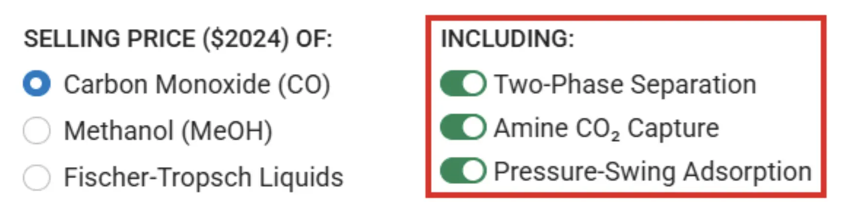
To alter the configuration of the process flow diagram or the target product, toggle between products and back-end separation blocks using the settings in the top-right corner of the homepage. Note: Separation options vary by product. When methanol or Fischer Tropsch liquids are selected as the final product, the unit operations utilized for separation are fixed, displaying only two-phase separation and amine CO₂ capture.

The heart of the tool and its analysis capabilities lies in the Data Inputs section, located in the left margin. In this section, more than 20 inputs can be manipulated across categories of electrolyzer technical performance, scale and market assumptions, and financial calculation parameters. By default, the tool provides initial estimates for each variable corresponding approximately to the current state of the art for CO₂ to CO electrolysis performance and/or market conditions. If you are unfamiliar with some parameters or uncertain about their impact, the default values provide a good starting point. The acceptable range for each parameter is shown below its label. For more information about individual parameters, refer to the assumptions and definitions.

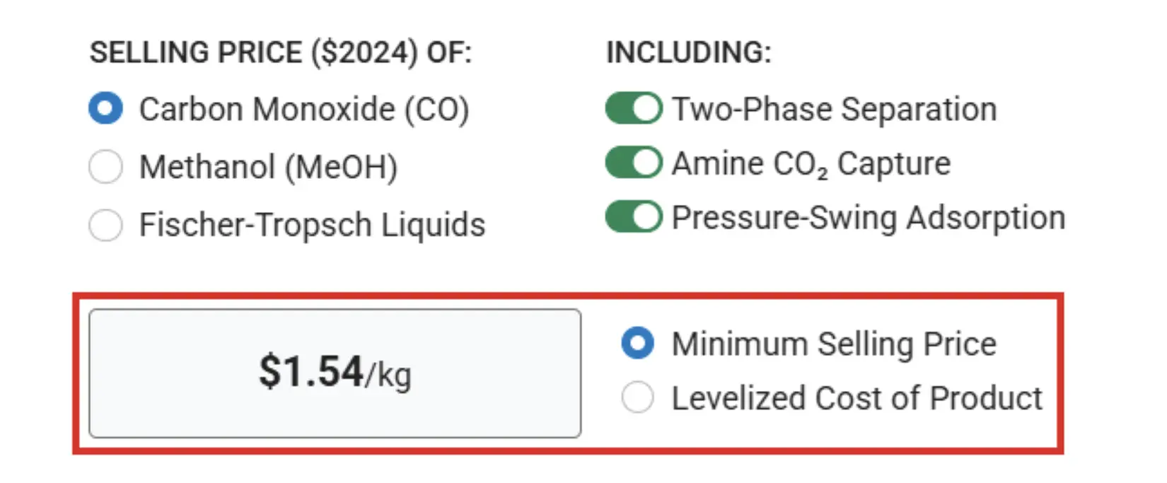
As data inputs are modified, the product selling price, listed in terms of $/kg (or $/GGE for FT-Liquids), automatically recalculates at the top of the page. The product selling price may be displayed using one of two techno-economic analysis methodologies: Minimum Selling Price or Levelized Cost of Product. For information about the distinction between these two methods, refer to the assumptions and definitions.

Cost Breakdown Chart

When data inputs are finalized and modifications to the process flow diagram are complete, this visualization shows the impacts of key areas on the carbon monoxide selling price. The key cost drivers are normalized in terms of $/kg CO and color-coded by category across capital, variable operations and maintenance (O&M), fixed O&M, and feedstock costs. Note: Cost breakdown values are provided only for the core CO₂ to CO electrochemical step and do not include downstream processes specific to upgrading to methanol or FT-Liquids (if selected).

OPEX/CAPEX Costs

Raw numerical values are provided for major operating expenditures (OPEX) and capital expenditures (CAPEX) based on data inputs in the Process Flowchart tab. Note: OPEX/CAPEX costs are provided only for the core CO₂ to CO electrochemical step and do not include downstream upgrading to methanol or FT-Liquids (if selected).

Life Cycle Inventory

Based on data inputs, this tab displays an estimated inventory of the major material and energy flows across the system. The CO₂ intensity associated with each material or energy flow is tabulated, and the impact on net carbon flows is calculated. Users may also create a custom blend of U.S.-based electricity by manipulating the source of energy used in the analysis.

For more information about life cycle inventory calculations, refer to the assumptions and definitions. Note: Life-cycle inventory values are provided only for the core CO₂ to CO electrochemical step and do not include downstream upgrading to methanol or FT-Liquids (if selected).

Monte Carlo

The Monte Carlo tab allows for personalized uncertainty analysis and assesses the impact of specific variables across up to 10,000 randomized simulations.

In the Monte Carlo tab:

1. Provide the number of simulations desired between 100 and 10,000.

2. Select the target parameters to vary.

3. Provide the minimum and maximum allowed values for each variable in the study.

4. Click Run Simulations.

The tool will initiate the Monte Carlo analysis. For each run, the model will default to the parameters listed in the Data Inputs section of the Process Flowchart, except for the user-defined parameters on the Monte Carlo tab. For these select parameters, the code will randomly generate a value between the listed minimum and maximum value, assuming a flat distribution. This process is repeated for the total number of simulations listed, and a histogram of the observed range of calculated selling prices is populated.

Once the histogram is populated, click on its individual bars to see the results of each "bin" of data. This provides information about what combination of parameters give rise to a specific range of selling prices and may be useful to inform target setting. The Monte Carlo analysis is compatible with any of the three target products.

Sensitivity Plot

The Sensitivity Plot assesses how two parameters simultaneously affect selling price and the magnitude of their correlation. At the bottom of the Sensitivity Plot tab, select two parameters and enter the target range to evaluate for each. Similar to the Monte Carlo analysis, the sensitivity plot is compatible with any of the three target products, and all other variables are held constant based on the values provided in the Data Inputs section. Once the data is input and the "Recalculate" button is clicked, the displayed heat map will show how product selling price varies as the two targeted metrics range between their min and max values.